
- 9 May 2024
- Paul Clarke
- Case Studies
University Marketing Funnel
The Marketing Funnel for University Undergraduate Students describes how Prospects (many thousands) are converted into Applicants with offers, and then into enrolled students who are finally registered in the Census count at the end of the first term (which determines tuition fee income).
This Blog
We at FiguringOutData.com are Data Analytics Specialists tasked with using data to boost performance at each stage in the Applicant Funnel for one of the UK’s middle-ranking Universities.
In this blog we look back at the first stage in the funnel (Prospects) for the 24/25 Academic Year and describe how we used Data Science to help attract as any Prospects as possible.
Maximising counts at each stage
To be sure of meeting the target set for the Census count, the number progressing between each stage needs to be as large as possible.
Mixed Channel Marketing will be needed. E.g. Paid Search with well researched keywords might be central to attracting Prospects and turning them into Applicants, whereas highly personalised emails might be vital for turning Offers into Offers Accepted.
Finding the optimal mix of channels
At each stage in the University Marketing Funnel there will be an optimal mix of inputs and activities that together exercise the greatest influence over the outcomes.
An Econometric Model is used to find that optimal mix. Once it is found the model can then show how to distribute spend across those inputs and activities for the greatest return on investment.
Stage 1 Prospects
In the first stage in the funnel we have sought to maximise the number of Prospects – on the basis that more Prospects should translate into more Applications and Offers, which in turn will translate into more Offers Accepted and Enrolments etc.
We used ‘Page Views through Searches’ to represent engagement by Prospects.
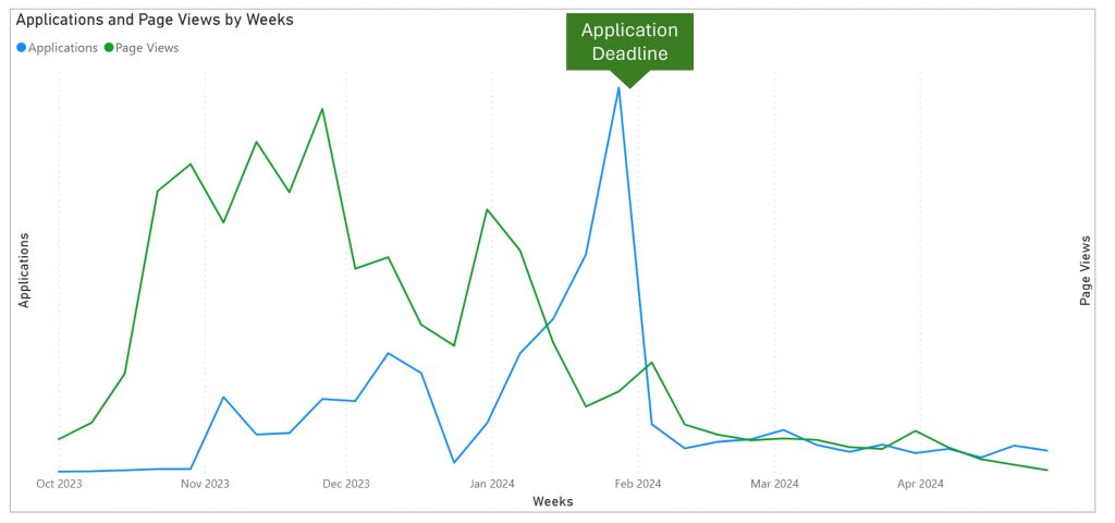
Figure 1 below compares Prospects and Applications up to the Universities and Colleges Admissions Service (UCAS) deadline, and then to the day of writing. (The spike in Applications is caused by the receipt of Applications made through UCAS – as distinct from those made directly to the University. The actual submission date for a UCAS application is not available).
To maximise the number of Prospects we needed to first know how the different inputs and activities influence Page Views through Searches. This involved comparing Page Views with factors such as:
- The number and effectiveness of Social Media Posts.
- The number of Blogs published and the length of time they remained published.
- Other Marketing Activities – e.g. Marketing Emails, SMS & Chat activity.
- The visibility of Keywords used in SEO and Paid Advertising (which in turn influence the visibility of the Domain as a whole).
Figures 2 to 5 below provide visualisations for each comparison.
1. Social Media Posts
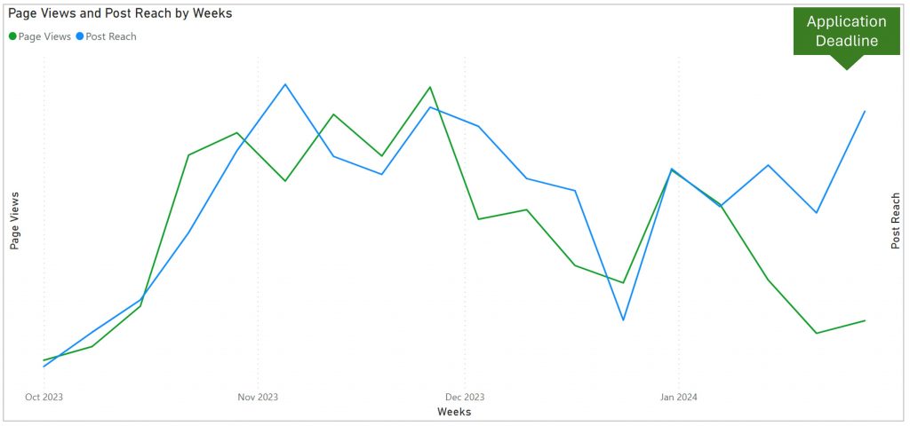
Figure 2 below compares Page Views with Meta Post Reach in the period leading up to the Application Deadline.
2. The number of and length of time Blogs are published
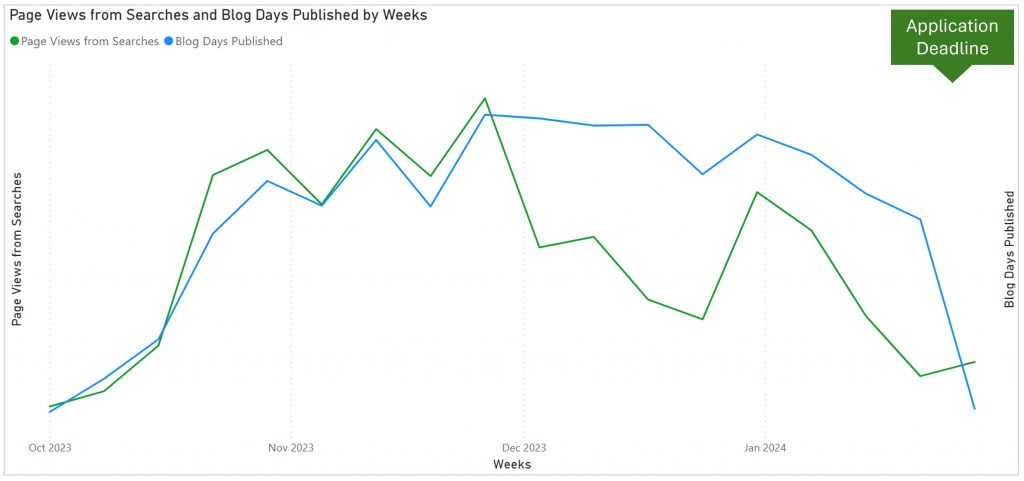
Figure 3 below compares Page Views with Blog Days Published. This is the number of Blogs published multiplied by the number of days each is published (e.g. 1 blog published for 7 days = 7 Blog Days).
3. Other Marketing Activities
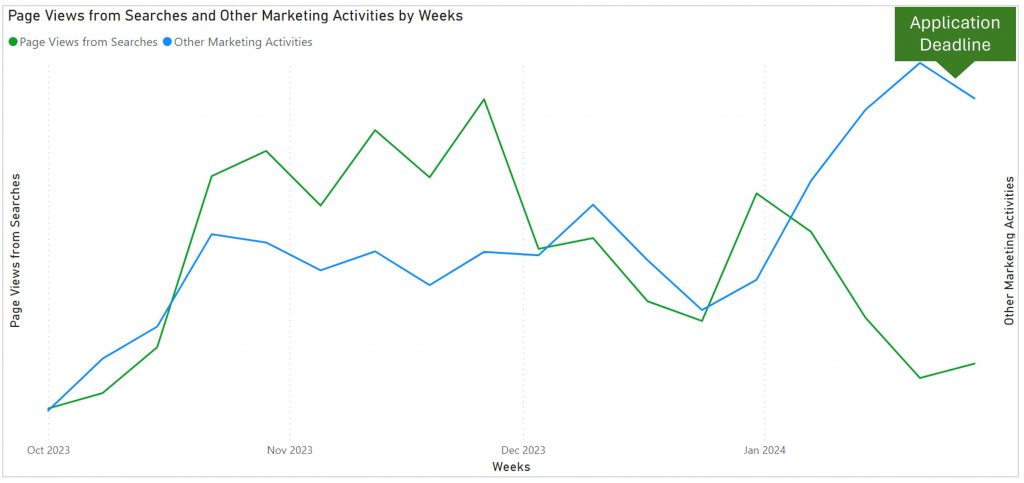
Figure 4 below compares a count of other Marketing Activities with Page Views. These include emails, on-line Chat & SMS conversations.
4. Keyword Visibility
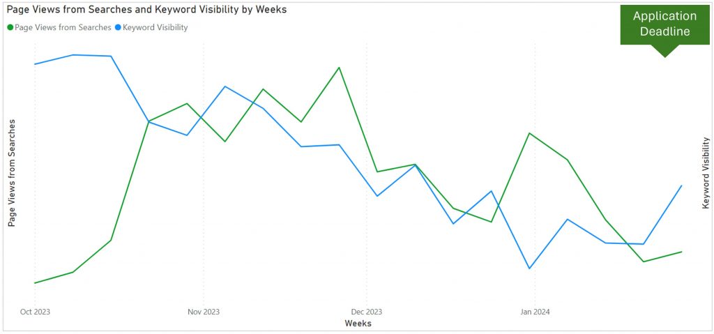
Figure 5 below shows how the average visibility for the top 100 performing Keywords compare with the Page Views at Figure 1.
Although Keyword Visibility influences Page Views from Searches, it also determined by Page Views. Its use as a predictor for Page Views was, therefore, limited.
Correlations with Page Views
The charts above give some insight into the factors that do most to influence Page Views from Searches. In Figure 2, for example, the line representing Meta Posts follows closely the count of Page Views up to a point a couple of weeks before the deadline.
This indicates that a level of correlation exists between the two that might allow Meta Posts to serve as predictor for Page Views.
This is also the case for Blog Days shown in Figure 3, and the Other Marketing activities at Figure 4.
Other factors at work
A feature common across Figures 1 to 4 is that, for the first half of the Stage 1 period, there is a good level of correlation between each factor and Page Views. However, it then weakens in the second half. This suggests that other factors were coming into play which are not included in the model so far.
In January, for example, Page Views decline just as Direct Applications start to increase sharply (Figure 1). This might suggest that, as more applications were submitted, fewer searches were then needed and fewer Page Views took place.
Turning Correlations into Coefficients
To act as a predictor for Page Views a mathematical equation is needed that links the factors above with Page Views.
The simplest approach is to use the average count for Blog Days over a period of time as the predictor for Page Views e.g.
Page Views = a x Average(Blog Days).
The letter ‘a’ is a coefficient designed to reduce the error between the actual count of Page Views and the predicted count to a minimum. This ‘residual error’ will, however, be significant.
A less simple, but more accurate approach is to find an equation such as:
Page Views = a x Blog Days + b
The coefficient ‘a’ now represents how many additional Page Views are gained for every additional Blog Day, and ‘b’ (called the Intercept) represents the static number which must then be added to reduce the residual error to a minimum.
A statistical approach called Linear Regression can establish whether such an equation is possible, and then identify the Coefficient and Intercept. Applying Linear Regression to the numbers used in Figure 2 (Blog Days) we get the following equation:
Page Views = 150 x Blog Days + 138,400
This suggests that, for each additional Blog Day, Page Views will increase by 150. Should there be zero Blog Days we would still achieve 138k Page Views.
We are however using a linear equation with just one predictor variable, when we know that other influences are at work. There will, therefore, still be a significant residual error albeit lower than that incurred using just the Blog Day average as a predictor (approx. 50% lower).
If we include Posts as well as Blog Days in the regression algorithm we obtain the following equation:
Page Views = 118 x Blog Days + 6 x Posts - 15,114
This shows the change in Page Views for each additional Blog Day and for each Post (118 + 6 = 124).
This is less than the increase in 150 under the equation for Blog Days on its own. The residual error however reduces further (by another 10%) indicating that predictions from the equation will be more accurate.
(There are a number of caveats plus important additional detail which are not covered here. This example is simply to illustrate the predictive methods used in the Econometric Model for Stage 1).
How these relationships are being used
These relationships were used firstly as inputs into an Econometric Model that could calculate the spend needed to deliver a set number of Prospects and Applications.
They were used secondly to help optimise all the inputs for the greatest number of Prospects. E.g. when Other Activities (Figure 4) were included in the regression algorithm they were revealed to be far less influential at delivering Page Views than the Blog Days and Posts in play at the same time.
This meant that money could be saved by reducing Other Activities without any detriment to the number of Prospects.
These relationships are now being used to remind all the Content Producers of the value of their work. Prospects will keep coming only if high quality Blogs and Posts continue to be produced.
By letting Content Producers know exactly how many additional Prospects are gained with each Blog and Post we are encouraging them to not only keep going, but to also strive to beat the benchmarks for performance that have now been set.
Stage 2 – Applicants and Offers
This stage is well underway with as many Applications as possible being translated into Offers.
The Econometric Model for this stage is focused upon Offers rather than Prospects.
We know already that the influences over the number of Offers made are to do with the Applicants themselves and the quality of their Applications, as well as the resources available and the time taken to review each Application.
All being well, when the Model for the stage is complete, we will be able to place the story for Stage 2 alongside the story told here about Stage 1.
